Hello WOLF
A good way to start working within the WOLF framework is by taking a look to the provided hello WOLF example.
Install and run
Download and compile WOLF core (a sistem-wide installation is not necessary at this point)
Before actually compiling, make sure you have the
BUILD_DEMOSoptionON, e.g. via ccmake:cd [wolf]/build/ ccmake .. <set BUILD_DEMOS to ON> make
or directly via cmake:
cd [wolf]/build/
cmake -DBUILD_DEMOS=ON ..
make
Execute the
hello_wolfdemocd [wolf]/bin ./hello_wolf
Execute the
hello_wolf_autoconfdemo (see below for explanations)cd [wolf]/bin ./hello_wolf_autoconf
Read on to understand the demo.
Problem statement
This example considers a planar robot with a range-and-bearing sensor ‘S’ mounted on a support arm at its front-left corner, looking forward. There are three landmarks in the environment. The robot will perform two motion steps, and so the trajectory will be composed of three keyframes. The following sketch illustrates the setup,
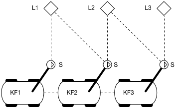
Robot performing a straight trajectory and observing 3 landmarks with its sensor
The image above represents the robot performing a straight trajectory. At every position the robot is able to see one (or more) of the represented landmarks ‘L’. The following is a more abstract representation of the same setup,
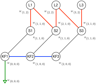
Sketch with the 3 robot kerframes, the 3 resulting sensors and the 3 landmarks positions
From the sketch and image above we can extract the following information:
The robot has two sensors
The odometry sensor acts as the robot reference frame, so its extrinsics are (x,y, theta) = (0,0, 0)
The range-and-bearing sensor is mounted at pose (1,1, 0) w.r.t. the robot’s origin
Keyframes have ids ‘1’, ‘2’, ‘3’
All Keyframes look East, so all orientations have theta = 0
Keyframes are at poses (0,0, 0), (1,0, 0), and (2,0, 0)
The resulting R&B sensor poses in world frame are (1,1, 0), (2,1, 0), and (3,1, 0)
We set a prior at (0,0, 0) on KF1 to render the system observable
Landmarks have ids ‘1’, ‘2’, ‘3’
Landmarks are at positions (x,y) = (1,2), (2,2), (3,2)
Not all landmarks are observed from all keyframes, but a only subset
Observations have ranges 1 or sqrt(2)
Observations have bearings pi/2 or 3pi/4
The landmarks observed at each keyframe are as follows (R is range, B is bearing):
KF1: L1 (R=1.0m, B=pi/2)
KF2: L1 (R=1.414m, B=3pi/4) and L2 (R=1.0m, B=pi/2)
KF3: L2 (R=1.414m, B=3pi/4) and L3 (R=1.0m, B=pi/2)
The robot starts at (0,0, 0) with a map with no previously known landmarks.
At each keyframe, the robot does:
Create a motion factor to the previous keyframe
Measure some landmarks. For each measurement,
If the landmark is unknown, add it to the map and create an observation factor
If the landmark is known, create an observation factor
After 3 keyframes, the problem to solve corresponds to the following factor graph,
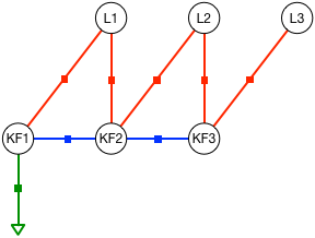
Factor graph of the problem of three keyframes and three landmarks above. Green: absolute prior factor. Blue: motion factors from odometry. Red: landmark observation factors from the R&B sensor.
This problem is solved and robot poses and landmark positions are optimized. For the sake of illustrating the optimization mechanisms, the effect of the initial guess, and other aspects of a graph-SLAM problem, this demo optimizes twice:
First, using the exact values as initial guess for the solver
Second, using random values far from the solution
Since we do not inject noise to any of the measurements, both solutions must produce the same exact values as in the sketches above.
Optionally, the user can opt to self-calibrate the sensor’s orientation (see NOTE within the code around Line 151). The associated factor graph for the self-calibration problem is as follows,
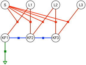
Factor graph of the problem of three keyframes and three landmarks,
with sensor self-calibration. The red factors related to landmark
observations also depend on the sensor calibration parameters S.
Explore the code
In this section we will go through the code bit by bit, explaining the
main functionality of each part. It might be helpful to have in hand the
WOLF tree when going thorugh
the hello_wolf.cpp and hello_wolf_autoconf.cpp code files.
Configuration of the robot platform and processing algorithms
The first section of the file sets the Hardware branch of the WOLF problem, that is,
The robot sensors
The data processors – usually one per sensor
then sets the initial robot pose and covariance, and configures the solver. This leaves the system ready to start receiving and processing sensory data.
The hello_wolf demo comes in two different methods for configuring
the problem:
A plain hello_wolf.cpp file containing all the configuration parameters hard-coded.
A hello_wolf_autoconf.cpp file with autoconfiguration from YAML parameter files. This makes use of the WOLF autoconf feature, which allows you to change mostly all parameters without having to recompile WOLF.
Apart from the respective configuration sections, both files are exactly the same.
Hard-coded configuration: hello_wolf.cpp
This uses the hello_wolf.cpp file.
Headers
We start with the heading section
// wolf core includes
#include "core/common/wolf.h"
#include "core/ceres_wrapper/solver_ceres.h"
#include "core/sensor/sensor_odom.h"
#include "core/processor/processor_odom_2d.h"
#include "core/capture/capture_odom_2d.h"

// hello wolf local includes
#include "sensor_range_bearing.h"
#include "processor_range_bearing.h"
#include "capture_range_bearing.h"

using namespace Eigen;
This basically advances us that the system will work with 2D odometry and range-and-bearing sensing.
Some of these includes come from wolf core. Others are specific to this application.
We are also using Ceres as the solver.
Problem properties
This problem is represented in 2 dimensions:
using namespace wolf;

// Wolf problem
ProblemPtr problem = Problem::create(2);
Optimizer options
We use the Ceres solver. Some of its options are required to be set. See the Ceres documentation for documentation of its meanings. Since in this demo, solver will not be executed in a thread, the period will not be used.
// Solver
YAML::Node params_solver;
params_solver["period"]                      = 1;
params_solver["verbose"]                     = 2;
params_solver["interrupt_on_problem_change"] = false;
params_solver["max_num_iterations"]          = 1000;
params_solver["n_threads"]                   = 2;
params_solver["parameter_tolerance"]         = 1e-8;
params_solver["function_tolerance"]          = 1e-8;
params_solver["gradient_tolerance"]          = 1e-9;
params_solver["minimizer"]                   = "levenberg_marquardt";
params_solver["use_nonmonotonic_steps"]      = false;
params_solver["compute_cov"]                 = false;
SolverCeresPtr ceres = std::static_pointer_cast<SolverCeres>(SolverCeres::create(problem, params_solver));
Sensors and processors properties
A typical scheme in robotics localization is to have sensors with which to integrate motion (by means of IMU integration, encoders in a wheeled robot, 2D odometry, etc.) and additionally, to have other sensors to observe the environment, thus providing the means to minimize or cancel motion drift, as well as mapping this environment.
All sensors involved in the localization problem, together with the algorithms taking care of the data they provide, must be added to the problem. This constitutes the Hardware branch of the WOLF tree.
In the hello
WOLF
example, we compute a 2D odometry. We add an odometry sensor to the
problem using the function
installSensor.
The parameters are, respectively, the sensor type, a given name for the
sensor, the sensor states and others.
In this case, the sensor states do not include intrinsic states.
As for the extrinsics (keys P, O), this sensor assumes that the odometry is computed at the
origin of the robot (see value fields).
Also, the states are set as static, i.e. will not change in time (see dynamic fields),
and fixed, i.e. will not be estimated (see prior/mode fields).
// Sensor odometer 2d
YAML::Node params_sen_odo;
params_sen_odo["type"]                         = "SensorOdom2d";
params_sen_odo["name"]                         = "Sensor Odometry";
params_sen_odo["states"]["P"]["value"]         = Vector2d::Zero();
params_sen_odo["states"]["P"]["prior"]["mode"] = "fix";
params_sen_odo["states"]["P"]["dynamic"]       = false;
params_sen_odo["states"]["O"]["value"]         = Vector1d::Zero();
params_sen_odo["states"]["O"]["prior"]["mode"] = "fix";
params_sen_odo["states"]["O"]["dynamic"]       = false;
params_sen_odo["enabled"]                      = true;
params_sen_odo["k_disp_to_disp"]               = 0.1;
params_sen_odo["k_disp_to_rot"]                = 0.1;
params_sen_odo["k_rot_to_rot"]                 = 0.1;
params_sen_odo["min_disp_var"]                 = 1;
params_sen_odo["min_rot_var"]                  = 1;
params_sen_odo["omnidirectional"]              = false;

SensorBasePtr sensor_odo = problem->installSensor(params_sen_odo);
std::cout << "sensor_odo created\n";
The sensory data can be processed using different algorithms. These algorithms are implemented in the so-called Processors.
We first define some parameters for the 2D odometry processor. The processor is added to the problem by using the method called installProcessor. Notice that we associate the processor to the sensor by passing the sensor name as a parameter.
// Processor odometer 2d
YAML::Node params_prc_odo;
params_prc_odo["type"]                               = "ProcessorOdom2d";
params_prc_odo["name"]                               = "Processor Odometry";
params_prc_odo["sensor_name"]                        = "Sensor Odometry";
params_prc_odo["time_tolerance"]                     = 0.1;
params_prc_odo["keyframe_vote"]["voting_active"]     = true;
params_prc_odo["keyframe_vote"]["max_time_span"]     = 999;
params_prc_odo["keyframe_vote"]["max_dist_traveled"] = 0.95;  // Will make KFs automatically every 1m displacement
params_prc_odo["keyframe_vote"]["max_angle_turned"]  = 999;
params_prc_odo["keyframe_vote"]["max_cov_det"]       = 999;
params_prc_odo["keyframe_vote"]["max_buff_length"]   = 999;
params_prc_odo["state_provider"]                     = true;
params_prc_odo["state_provider_order"]               = 1;
params_prc_odo["unmeasured_perturbation_std"]        = 0.001;
params_prc_odo["debug_verbose_level"]                = "none";
params_prc_odo["apply_loss_function"]                = false;

ProcessorBasePtr processor = problem->installProcessor(params_prc_odo);
std::cout << "processor created\n";
We now specify the R&B (i.e., Range & Bearing, do not confuse with Rythm&Blues, which would be a very different thing) sensor and processor.
Once we have the parameters for sensor and processor, we use
installSensor and installProcessor as before.
Notice that these sensor and processor classes have been created for didactic purposes in hello_wolf, and all related files are inside the hello WOLF folder.
// Sensor Range and Bearing
YAML::Node params_sen_rb;
params_sen_rb["type"]                         = "SensorRangeBearing";
params_sen_rb["name"]                         = "Sensor Range Bearing";
params_sen_rb["states"]["P"]["value"]         = Vector2d::Zero();
params_sen_rb["states"]["P"]["prior"]["mode"] = "fix";
params_sen_rb["states"]["P"]["dynamic"]       = false;
params_sen_rb["states"]["O"]["value"]         = Vector1d::Zero();
params_sen_rb["states"]["O"]["prior"]["mode"] = "fix";
params_sen_rb["states"]["O"]["dynamic"]       = false;
params_sen_rb["enabled"]                      = true;
params_sen_rb["noise_range_metres_std"]       = 0.1;
params_sen_rb["noise_bearing_degrees_std"]    = 1.0;

SensorBasePtr sensor_rb = problem->installSensor(params_sen_rb);
std::cout << "sensor_rb created\n";

// Processor Range and Bearing
YAML::Node params_prc_rb;
params_prc_rb["type"]                = "ProcessorRangeBearing";
params_prc_rb["name"]                = "Processor Range Bearing";
params_prc_rb["sensor_name"]         = "Sensor Range Bearing";
params_prc_rb["voting_active"]       = false;
params_prc_rb["time_tolerance"]      = 0.01;
params_prc_rb["debug_verbose_level"] = "none";
params_prc_rb["apply_loss_function"] = false;

ProcessorBasePtr processor_rb = problem->installProcessor(params_prc_rb);
std::cout << "processor_rb created\n";
We completed the Hardware branch of the WOLF tree, using a configuration method hard-coded in the main cpp file.
Initial robot conditions
Next, and before beginning to process sensory data, wet need to indicate
the initial robot pose. This we do with the method Problem::emplaceFirstFrame.
Also, we set this first frame as the origin of the odometry processor with the method ProcessorMotion::setOrigin()
(to do so, we have to cast its pointer from ProcessorBasePtr to ProcessorMotionPtr).
// Initialize
TimeStamp  t(0.0);  // t : 0.0
YAML::Node params_first_frame;
params_first_frame["P"]["value"]               = Vector2d::Zero();
params_first_frame["P"]["prior"]["mode"]       = "factor";
params_first_frame["P"]["prior"]["factor_std"] = Vector2d::Constant(sqrt(0.1));
params_first_frame["O"]["value"]               = Vector1d::Zero();
params_first_frame["O"]["prior"]["mode"]       = "factor";
params_first_frame["O"]["prior"]["factor_std"] = Vector1d::Constant(sqrt(0.1));

FrameBasePtr KF1 = problem->emplaceFirstFrame(t,
                                              params_first_frame);  // KF1 : (0,0,0)
std::static_pointer_cast<ProcessorMotion>(processor)->setOrigin(KF1);
At this point, the problem set up is complete. Congratulations!
Automatic configuration with YAML: hello_wolf_autoconf.cpp
This uses the hello_wolf_autoconf.cpp file.
WOLF provides an WOLF autoconf feature that places all user data for configuration outside of the
compiled code using YAML files.
This feature includes YAML files verification using the yaml-schema-cpp library, and produces a final YAML::Node containing
whole WOLF specification that is used to build the problem.
Headers
We start with the header,
// wolf core includes
#include "core/common/wolf.h"
#include "core/ceres_wrapper/solver_ceres.h"
#include "core/solver/factory_solver.h"
#include "core/capture/capture_odom_2d.h"
#include "core/processor/processor_motion.h"

// hello wolf local includes
#include "capture_range_bearing.h"

using namespace Eigen;
Comparing to the header section of the plain cpp file above, we notice that:
we removed the sensors and processors headers. We only require the captures headers, as in such Captures is where we are going to store the sensory data to be processed. And the
processor_motionto be able to set the origin of the odometry processor.We added the solver factory header, which is needed to create the solver object.
Note
In a real robotics application, only headers to files in WOLF core should remain. This allows us to write generic code using only objects of the base classes in WOLF core. All the code for the derived classes is loaded at runtime through the usage of WOLF plugins, as required by the YAML configuration files.
In the hello_wolf case, data processing requires the explicit
creation of derived Capture objects,
and therefore the headers capture_odom_2D.h and
capture_range_bearing.h for the derived Capture classes are
necessary. See this section
below for
more details.
When using a robotics environment such as ROS2, these headers will also be removed from the main application. See the ROS2 integration to learn how to do it.
YAML configuration files
We specify the path to a YAML configuration
file
containing all that is needed to set up the hello_wolf demo,
using namespace wolf;

WOLF_INFO("======== CONFIGURE PROBLEM =======");

// Config file to parse. Here is where all the problem is defined:
std::string wolf_path   = _WOLF_CODE_DIR;
std::string config_file = wolf_path + "/demos/hello_wolf/yaml/hello_wolf_config.yaml";
Explore the YAML file of the hello_wolf demo here. A copy is reproduced below,
problem:

  dimension:            2               # space is 2d
  frame_structure:      "PO"            # keyframes have position and orientation

  first_frame:
    P:
      value: [0,0]
      prior:
        mode:               "factor"
        factor_std: [0.31, 0.31]
    O:
      value: [0]
      prior:
        mode:               "factor"
        factor_std: [0.31]

  tree_manager:
    type: "none"

solver:
  type: SolverCeres
  plugin: core
  max_num_iterations: 100
  verbose: 0
  period: 0.2
  interrupt_on_problem_change: false
  n_threads: 2
  compute_cov: false
  minimizer: levenberg_marquardt
  use_nonmonotonic_steps: false         # only for levenberg_marquardt and DOGLEG
  parameter_tolerance: 1e-6
  function_tolerance: 1e-6
  gradient_tolerance: 1e-10

sensors:

  - type:               "SensorOdom2d"
    plugin:             "core"
    name:               "sen odom"
    follow:             "sensor_odom_2d.yaml"         # config parameters in this file

  - type:               "SensorRangeBearing"
    plugin:             "core"
    name:               "sen rb"
    noise_range_metres_std: 0.2                       # parser only considers first appearence so the following file parsing will not overwrite this param
    follow:             sensor_range_bearing.yaml     # config parameters in this file

processors:

  - type:               "ProcessorOdom2d"
    plugin:             "core"
    name:               "prc odom"
    sensor_name:        "sen odom"                    # attach processor to this sensor
    follow:             processor_odom_2d.yaml        # config parameters in this file

  - type:               "ProcessorRangeBearing"
    plugin:             "core"
    name:               "prc rb"
    sensor_name:        "sen rb"                      # attach processor to this sensor
    follow:             processor_range_bearing.yaml  # config parameters in this file
In this file, you should be able to identify the same parameters that
were entered in the hard-coded cpp version above. To do so, see that for
each sensor, and for each processor, you find new YAML files after the
tag follow:. This indicates the parser that further parameters are
to be found in such new files. For reference, we reproduce here the
files sensor_range_bearing.yaml,
noise_range_metres_std:     0.1
noise_bearing_degrees_std:  0.5
apply_loss_function: true

states:
  P:
    prior:
      mode: fix
    value: [1,1]
    dynamic: false
  O:
    prior:
      mode: fix
    value: [0]
    dynamic: false
and processor_range_bearing.yaml,
time_tolerance:       0.1

keyframe_vote:
  voting_active:      true

debug_verbose_level: "none"

apply_loss_function: true
Having the sensor and processor parameters separated from the main YAML file is very useful. You may have a collection of sensors already calibrated, and a collection of algorithms already tuned, and you may use them in different robots in different projects. Their associated YAML files will be reused across these projects.
See that even if you re-use parameter files, you can overwrite some or
all of their parameters in your particular projects.
At this time,
only preceding overwrites work: you have to write the parameter you
want to overwrite before the follow: tag. See in the main YAML file
the two consecutive lines achieving this effect:
[...]
  noise_range_metres_std: 0.2                           # first appearence: this value will prevail
  follow: hello_wolf/yaml/sensor_range_bearing.yaml     # noise_range_metres_std in here is ignored
[...]
Autoconfiguring the problem and the solver
We are now ready to create the problem and the solver. The problem will contain all the Hardware branch of the WOLF tree and the problem initialization.
For this, we just have to provide the configuration YAML file path to the static
autoSetup() method of Problem and SolverManager, respectively.
Before creating the problem or the solver, the autoSetup will firstly validate
the YAML file content (missing parameters, wrong types, etc.) and raise the corresponding error message, eventually.
To perform the YAML validation, we have to provide a list of paths where
the installed schema files are (autoSetup last argument).
Specifically, the SolverManager::autoSetup() also requires the pointer of the WOLF problem.
// Wolf problem: Build the Hardware branch of the wolf tree from the config yaml file
ProblemPtr problem = Problem::autoSetup(config_file, {wolf_path});

// Solver: Create a Solver Ceres from the config yaml file
SolverManagerPtr ceres = SolverManager::autoSetup(problem, config_file, {wolf_path});
We also recover pointers to the sensors which will be needed later on.
// recover sensor pointers and other stuff for later use (access by sensor name)
SensorBasePtr sensor_odo = problem->findSensor("sen odom");
SensorBasePtr sensor_rb  = problem->findSensor("sen rb");
Now, we can apply the first frame options. In a typical robotics application, this would be automatically performed when the first capture is processed taking this capture timestamp as the first frame timestamp. In this demo, we trigger it manually:
// Apply first frame options
TimeStamp    t(0.0);
FrameBasePtr KF1 = problem->applyFirstFrameOptions(t);
At this point, the configuration is done. We print the WOLF tree for verification purposes.
// Print problem to see its status before processing any sensor data
problem->print(4, 0, 1, 0);
The printed tree should look like this (side comments added here for reference),
Wolf tree status ------------------------
Hardware                                  -- Hardware branch: robot and software characteristics
  Sen1 SensorOdom2d "sen odom"            -- Sensor ID, type, and name
    Fix,     x = ( 0 0 0 )                  -- Extrinsics are fixed, at the origin
    PrcM1 ProcessorOdom2d "prc odom"      -- ProcessorMotion ID, type, and name
  Sen2 SensorRangeBearing "sen rb"        -- Sensor ID, type, and name
    Fix,     x = ( 0 1 1 )                  -- Extrinsics are fixed, pose (see sketch at top of page)
    Prc2 ProcessorRangeBearing "prc rb"   -- ProcessorTracker ID, type, and name
Trajectory                                -- Trajectory branch: time-dependent information produced as robot evolves through time
  Frm1 OP ts = 0.000000000                -- Frame ID, state keys (O: orientation, P: position), timestamp = 0
    Est,     x = ( 0 0 0 )                  -- State is estimated, values
Map                                       -- Map branch: environment information produced as robot evolves through time. Map is still empty!
-----------------------------------------
that is, we have the sensors and processors, an initial frame at the origin of coordinates. Since the robot did not start moving yet, we observe no other frame and an absolutely empty map.
Self-calibration
You are free to activate self-calibration of the extrinsic parameters of the R&B sensor. You do this by fixing / unfixing these sensor parameters. This can be done in two ways:
Specifying the sensor state
priordifferent thanfix(eitherinitial_guessorfactor).Unfixing the state, hard-coded in the cpp file (either
hello_wolf.cpporhello_wolf_autoconf.cpp)
Try uncommenting the following lines to unfix the sensor states:
// SELF CALIBRATION ===================================================
// These few lines control whether we calibrate some sensor parameters or not.

// SELF-CALIBRATION OF SENSOR ORIENTATION
// Uncomment this line below to achieve sensor self-calibration (of the orientation only, since the position is not
// observable)
// sensor_rb->getO()->unfix();
Note
For the type of setup and the trajectory that we performed, only the sensor orientation is observable. So unfixing the sensor orientation should lead to a proper observation of the sensor orientation, The sensor position is however not observable. This means that unfixing the sensor position should yield aberrant results. You can however try and see what comes out,
Simulating and Capturing data
For didactical purposes and simplicity, in this hello_wolf application we simulate motion and sensor data inside the main file.
We first configure a few basic variables. These are related to motion data on one hand, and landmark observations on the other hand.
Motion data comes in the form of a 2-vector with forward motion (m) and turn (rad) increments. This vector is accompained by the respective covariances matrix.
Landmark observations come with a vector of landmakr IDs, a vector of ranges to these landmarks, and a vector of angles or bearings. These measurements will be computed from each robot pose according to the sketch at the top of this page. The uncertainty of these measurements is a parameter of the R&B sensor. The covariances matrix is computed internally by the R&B sensor at construction time, and fetched by the processor when required.
// CONFIGURE=====================================
// Motion data
Vector2d motion_data(1.0, 0.0);    // Will advance 1m at each keyframe, will not turn.
Matrix2d motion_cov = 0.1 * Matrix2d::Identity();

// landmark observations data
VectorXi ids;
VectorXd ranges, bearings;
Note
In a typical robotics framework, the code generating the data would remain outside of the estimation algorithm: sensors would capture data either from a real robot or from a simulation environment (such as Gazebo). Then, this data would be streamed in a way such that WOLF can access to it, e.g using ROS2. See the WOLF ROS2 Laser 2d Demo for such a realistic application.
Building the wolf problem with the simulated data
In this case, we just execute a fixed sequence of steps. This will produce the measurements with which we populate the WOLF tree.
In the first step, we just observe landmark no. 1. Please refer to
the sketch at the beginning of this page for the measured values of
range and bearing. With the measurements we create a
wolf::CaptureRangeBearing object, which is then processed,
// SET OF EVENTS =======================================================
std::cout << std::endl; WOLF_TRACE("======== START ROBOT MOVE AND SLAM =======")

// We'll do 3 steps of motion and landmark observations.

// STEP 1 --------------------------------------------------------------

// observe lmks
ids.resize(1); ranges.resize(1); bearings.resize(1);
ids         << 1;                       // will observe Lmk 1
ranges      << 1.0;                     // see drawing
bearings    << M_PI/2;
CaptureRangeBearingPtr cap_rb = std::make_shared<CaptureRangeBearing>(t,
                                                                      sensor_rb,
                                                                      ids,
                                                                      ranges,
                                                                      bearings);
cap_rb      ->process();                // L1 : (1,2)
Observe that all we have to do is create a Capture of the correct type,
and call capture->process(). WOLF takes care of all the rest.
Note
Notice that we are creating (a shared pointer to) an object of the
type CaptureRangeBearing. This is why the file
capture_range_bearing.h had to be included in the header. When
using ROS or other robotic management systems, this include will be
no longer required in the main file. Together with the autoconf
feature, this will allow us to write a main file that is generic for
any robotics application, regardless of the number and types of
sensor used.
See Further steps below for more information.
The second step starts by moving the robot to a new position, and then
observing landmarks 1 and 2,
// STEP 2--------------------------------------------------------------
t += 1.0; // t : 1.0

// motion
CaptureOdom2DPtr cap_motion = std::make_shared<CaptureOdom2D>(t, sensor_odo, motion_data, motion_cov);
cap_motion  ->process();      // KF2 : (1,0,0)
// observe lmks
ids.resize(2); ranges.resize(2); bearings.resize(2);
ids         << 1, 2;                    // will observe Lmks 1 and 2
ranges      << sqrt(2.0), 1.0;          // see drawing
bearings    << 3*M_PI/4, M_PI/2;
cap_rb      = std::make_shared<CaptureRangeBearing>(t, sensor_rb, ids, ranges, bearings);
cap_rb      ->process();      // L1 : (1,2), L2 : (2,2)
The third and last step moves the robot further, then observes landmarks
2 and 3,
// STEP 3--------------------------------------------------------------
t += 1.0; // t : 2.0

// motion
cap_motion  ->setTimeStamp(t);
cap_motion  ->process();      // KF3 : (2,0,0)
// observe lmks
ids.resize(2); ranges.resize(2); bearings.resize(2);
ids         << 2, 3;                    // will observe Lmks 2 and 3
ranges      << sqrt(2.0), 1.0;          // see drawing
bearings    << 3*M_PI/4, M_PI/2;
cap_rb      = std::make_shared<CaptureRangeBearing>(t,
                                                    sensor_rb,
                                                    ids,
                                                    ranges,
                                                    bearings);
cap_rb      ->process();          // L1 : (1,2), L2 : (2,2), L3 : (3,2)
At this point, we print the wolf tree again,
problem->print(1,0,1,0);
This is the outcome, clearily showing three keyframes and three landmarks. Their initial positions are those computed from the measurements. Since we did not inject any noise to these measurements, these positions exactly match the true positions – refer to the sketch at the beginning of this page.
P: wolf tree status ---------------------
Hardware
  S1 ODOM 2D "sen odom" -- 1p
    Extr [Sta]= ( 0 0 0 )
  S2 RANGE BEARING "sen rb" -- 1p
    Extr [Sta]= ( 1 1 0 )
Trajectory
  KF1 -- 3C
    Est, ts=0,   x = ( 0 0 0 )
  KF2 -- 2C
    Est, ts=1,   x = ( 1 0 0 )
  KF3 -- 2C
    Est, ts=2,   x = ( 2 0 0 )
  F4 -- 1C
    Est, ts=2,   x = ( 2 0 0 )
Map
  L1 POINT 2D
    Est,     x = ( 1 2 )
  L2 POINT 2D
    Est,     x = ( 2 2 )
  L3 POINT 2D
    Est,     x = ( 3 2 )
Solving the wolf problem with exact data
At this point and with non-noisy data, the solution to our problem must be exactly the same as the one we just introduced. Therefore, Ceres should perform one only iteration and return with a very low final cost or residual, and exactly the same optimal solution,
// SOLVE================================================================

// SOLVE with exact initial guess
WOLF_TRACE("======== SOLVE PROBLEM WITH EXACT PRIORS =======")
std::string report = ceres->solve(wolf::SolverManager::ReportVerbosity::FULL);
WOLF_TRACE(report);                     // should show a very low iteration number (possibly 1)
problem->print(1,0,1,0);
The report of the Ceres solver effectively certifies this,
Solver Summary (v 1.14.0-eigen-(3.2.92)-lapack-suitesparse-(4.4.6)-cxsparse-(3.1.4)-eigensparse-openmp-no_tbb)

                                     Original                  Reduced
Parameter blocks                           13                        9
Parameters                                 21                       15
Residual blocks                             8                        8
Residuals                                  19                       19

Minimizer                        TRUST_REGION

Sparse linear algebra library    SUITE_SPARSE
Trust region strategy     LEVENBERG_MARQUARDT

                                        Given                     Used
Linear solver          SPARSE_NORMAL_CHOLESKY   SPARSE_NORMAL_CHOLESKY
Threads                                     1                        1
Linear solver ordering              AUTOMATIC                        9

Cost:
Initial                          0.000000e+00
Final                            0.000000e+00
Change                           0.000000e+00

Minimizer iterations                        1
Successful steps                            1
Unsuccessful steps                          0

Time (in seconds):
Preprocessor                         0.000135

  Residual only evaluation           0.000000 (0)
  Jacobian & residual evaluation     0.003778 (1)
  Linear solver                      0.000000 (0)
Minimizer                            0.003847

Postprocessor                        0.000010
Total                                0.003991

Termination:                      CONVERGENCE (Gradient tolerance reached. Gradient max norm: 0.000000e+00 <= 1.000000e-10)
Solving with perturbed data
What we will do now is simulate an initial guess for the optimizer that is not at the true position. We do this by perturbing the state values in the WOLF tree: sensor parameters (only if they are estimated), keyframes and landmark positions are rewritten to new values:
// PERTURB initial guess
WOLF_TRACE("======== PERTURB PROBLEM PRIORS =======")
for (auto& sen : problem->getHardwarePtr()->getSensorList())
  for (auto& sb : sen->getStateBlockVec())
    if (sb && !sb->isFixed())
      // We perturb A LOT !
      sb->setState(sb->getState() + VectorXd::Random(sb->getSize()) * 0.5);
for (auto& kf : problem->getTrajectoryPtr()->getFrameList())
  if (kf->isKey())
    for (auto& sb : kf->getStateBlockVec())
      if (sb && !sb->isFixed())
        // We perturb A LOT
        sb->setState(sb->getState() + VectorXd::Random(sb->getSize()) * 0.5;
for (auto& lmk : problem->getMapPtr()->getLandmarkList())
  for (auto& sb : lmk->getStateBlockVec())
    if (sb && !sb->isFixed())
      // We perturb A LOT !
      sb->setState(sb->getState() + VectorXd::Random(sb->getSize()) * 0.5);

problem->print(1,0,1,0);
We now solve again. This time, Ceres must iterate several times to arrive at an optimum,
// SOLVE again
WOLF_TRACE("======== SOLVE PROBLEM WITH PERTURBED PRIORS =======")
report = ceres->solve(wolf::SolverManager::ReportVerbosity::FULL);
WOLF_TRACE(report);                     // should show a very high iteration number (more than 10, or than 100!)
problem->print(1,0,1,0);
This new solution can be shown using Problem::print(...) to converge
to the previous one,
P: wolf tree status ---------------------
Hardware
  S1 ODOM 2D "sen odom" -- 1p
    Extr [Sta]= ( 0 0 0 )
  S2 RANGE BEARING "sen rb" -- 1p
    Extr [Sta]= ( 1 1 0 )
Trajectory
  KF1 -- 3C
    Est, ts=0,   x = ( -4.4e-14 1.5e-11  2.6e-11  )
  KF2 -- 2C
    Est, ts=1,   x = ( 1       5.6e-11 5.6e-11 )
  KF3 -- 2C
    Est, ts=2,   x = ( 2       1.2e-10 6.5e-11 )
  F4 -- 1C
    Est, ts=2,   x = ( 2 0 0 )
Map
  L1 POINT 2D
    Est,     x = ( 1 2 )
  L2 POINT 2D
    Est,     x = ( 2 2 )
  L3 POINT 2D
    Est,     x = ( 3 2 )
In our case, the optimization report shows 12 iterations and a final cost in the order of 1e-20. Your case might be slightly different, for any reason, but not substantially different.
Computing and recovering covariances of the estimates
We can also recover the covariance of the estimates of all variables of interest,
// GET COVARIANCES of all states
WOLF_TRACE("======== COVARIANCES OF SOLVED PROBLEM =======")
ceres->computeCovariances(SolverManager::CovarianceBlocksToBeComputed::ALL_MARGINALS);
for (auto& kf : problem->getTrajectory()->getFrameList())
  if (kf->isKeyOrAux())
  {
    Eigen::MatrixXd cov;
    kf->getCovariance(cov);
    WOLF_TRACE("KF", kf->id(), "_cov = \n", cov);
  }
  for (auto& lmk : problem->getMap()->getLandmarkList())
  {
    Eigen::MatrixXd cov;
    lmk->getCovariance(cov);
    WOLF_TRACE("L", lmk->id(), "_cov = \n", cov);
  }
  std::cout << std::endl;
which returns three 3x3 covariance matrices for the KFs, and three 2x2 covariance matrices for the landmarks,
[trace][15:15:07] [hello_wolf_autoconf.cpp L237 : main] ======== COVARIANCES OF SOLVED PROBLEM =======
[trace][15:15:07] [hello_wolf_autoconf.cpp L244 : main] KF1_cov =
        0.01  3.18771e-19  5.83553e-19
 6.40769e-20         0.01 -2.51862e-18
 5.83553e-19 -2.51862e-18         0.01
[trace][15:15:07] [hello_wolf_autoconf.cpp L244 : main] KF2_cov =
 0.066609 0.0149901 0.0299834
0.0149901 0.0242264 0.0184509
0.0299834 0.0184509 0.0269031
[trace][15:15:07] [hello_wolf_autoconf.cpp L244 : main] KF3_cov =
 0.123218 0.0599637 0.0599669
0.0599637 0.0922575 0.0538048
0.0599669 0.0538048 0.0438061
[trace][15:15:07] [hello_wolf_autoconf.cpp L250 : main] L1_cov =
 0.0500761 -0.0200087
-0.0200087  0.0245307
[trace][15:15:07] [hello_wolf_autoconf.cpp L250 : main] L2_cov =
 0.0543637 -0.0457429
-0.0457429  0.0925619
[trace][15:15:07] [hello_wolf_autoconf.cpp L250 : main] L3_cov =
 0.0586512 -0.0752913
-0.0752913   0.253673
Finally, we print the wolf tree again, this time in full detail — see
the documentation of Problem::print().
WOLF_TRACE("======== FINAL PRINT FOR INTERPRETATION =======")
problem->print(4,1,1,1);
The outcome of this is reproduced below. A commented version of this outcome can be found in the last part of the source code file.
Observe that the map now contains three landmarks, and that their positions are exactly where they should be according to the sketch at the beginning of this page.
[trace][15:15:07] [hello_wolf_autoconf.cpp L254 : main] ======== FINAL PRINT FOR INTERPRETATION =======

P: wolf tree status ---------------------
Hardware
  S1 ODOM 2D "sen odom"
    Extr [Sta] = [ Fix( 0 0 ) Fix( 0 ) ]
    Intr [Sta] = [ ]
    pm1 ODOM 2D "prc odom"
      o: C6 -   KF3
      l: C8 -   F4
  S2 RANGE BEARING "sen rb"
    Extr [Sta] = [ Fix( 1 1 ) Fix( 0 ) ]
    Intr [Sta] = [ ]
    pt2 RANGE BEARING "prc rb"
Trajectory
  KF1  <-- c3
    Est, ts=0,   x = ( -4.4e-14 1.5e-11  2.6e-11  )
    sb: Est Est
    C1 POSE -> S-  <--
      f1 trk0 POSE  <--
        m = ( 0 0 0 )
        c1 POSE 2D --> A
    CM2 ODOM 2D -> S1 [Sta, Sta]  <--
      buffer size  :  0
    C4 RANGE BEARING -> S2 [Sta, Sta]  <--
      f2 trk0 RANGE BEARING  <--
        m = ( 1   1.6 )
        c2 RANGE BEARING --> L1
  KF2  <-- c6
    Est, ts=1,   x = ( 1       5.6e-11 5.6e-11 )
    sb: Est Est
    CM3 ODOM 2D -> S1 [Sta, Sta] -> OC2 ; OF1  <--
      buffer size  :  2
      delta preint : (1 0 0)
      f3 trk0 ODOM 2D  <--
        m = ( 1 0 0 )
        c3 ODOM 2D --> F1
    C7 RANGE BEARING -> S2 [Sta, Sta]  <--
      f4 trk0 RANGE BEARING  <--
        m = ( 1.4 2.4 )
        c4 RANGE BEARING --> L1
      f5 trk0 RANGE BEARING  <--
        m = ( 1   1.6 )
        c5 RANGE BEARING --> L2
  KF3  <--
    Est, ts=2,   x = ( 2       1.2e-10 6.5e-11 )
    sb: Est Est
    CM6 ODOM 2D -> S1 [Sta, Sta] -> OC3 ; OF2  <--
      buffer size  :  2
      delta preint : (1 0 0)
      f6 trk0 ODOM 2D  <--
        m = ( 1 0 0 )
        c6 ODOM 2D --> F2
    C9 RANGE BEARING -> S2 [Sta, Sta]  <--
      f7 trk0 RANGE BEARING  <--
        m = ( 1.4 2.4 )
        c7 RANGE BEARING --> L2
      f8 trk0 RANGE BEARING  <--
        m = ( 1   1.6 )
        c8 RANGE BEARING --> L3
  F4  <--
    Est, ts=2,   x = ( 2 0 0 )
    sb: Est Est
    CM8 ODOM 2D -> S1 [Sta, Sta] -> OC6 ; OF3  <--
      buffer size  :  1
      delta preint : (0 0 0)
Map
  L1 POINT 2D   <-- c2  c4
    Est,     x = ( 1 2 )
    sb: Est
  L2 POINT 2D   <-- c5  c7
    Est,     x = ( 2 2 )
    sb: Est
  L3 POINT 2D   <-- c8
    Est,     x = ( 3 2 )
    sb: Est
-----------------------------------------
This completes the introduction to WOLF through a simple stand-alone application. Again, Congratulations!
Further steps
This Hello WOLF application is not realistic mainly in two senses:
The data flow is rigidly coded in the main algorithm and cannot be applied to real robots. For this, additional procedures for real-time handling of events generated by the arrival of sensory data is necessary. A platform like ROS will come handy in this regard.
The data of the R&B sensor is already processed and contains the range and bearing measurements to landmarks. In reality, these measurements must be extracted from raw data. This is one fo the roles of the realistic processors in wolf.
These two aspects are addressed in the ROS WOLF demo, which we recommend you visit next.